Excel Guide to Lookups and Matching Cells

Excel Guide to Lookups and Matching Cells

Overview

Lookup functionality is undoubtedly one of the most heavily used features in Microsoft Excel. There are several functions or formulas used to look up Excel information. Today we will learn about some commonly used lookups and whether they can be used more effectively.

The most popular approach to lookup information is to use the VLOOKUP function. However, its wide popularity doesn’t necessarily make it appropriate to use in every situation. In fact, there are many occasions where another lookup formula fits much better.

Before we get into the superior lookup methods, let’s briefly discuss VLOOKUP.

Brief Overview of Vlookup

Let’s start by reviewing VLOOKUP’s structure

=VLOOKUP(VALUE TO MATCH, TABLE TO CHECK AGAINST, COLUMN TO RETURN, Approximate or Exact Match)

Let’s get an example of VLOOKUP in action:

=VLOOKUP(B15, $F$15: $G$21, 2, FALSE)

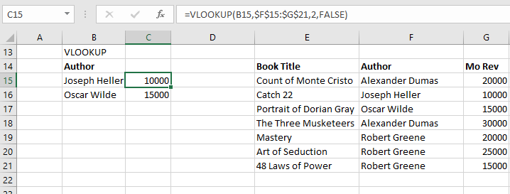
After dissecting the example above and examining the screenshot here are some observations:

Cell B15 contains the value we are seeking a match for.

The table range we have selected is F through G. Although E is technically part of the table we omitted it from the range because it doesn’t add value and will likely generate an error.

“2” refers to the column number to be returned once a corresponding match is identified. The column number counts columns starting with the first column in the table range select by the user.

The last segment of the formula determines whether the value returned is required to be an exact match (FALSE) or an approximate match (TRUE). In this example and most other cases, FALSE is the best result to prevent confusion. TRUE utilizes fuzzy logic to find the closest value which I’ve found to cause more harm than good.

The VLOOKUP above returns 10000 and 15000 since these are the values Corresponding with the authors in our lookup.

Notice in the above example, we didn’t use one of the authors with duplicate Novels. VLOOKUP against duplicates can return inaccurate results, we will later discuss a more suitable function. Or we can just identify and remove duplicate values.

Shifting away from VLOOKUP

VLOOKUP can be a great tool in your Excel troubleshooting toolbox for matching or looking up values. However, It shouldn’t be the default lookup method in these scenarios.

In many situations, other lookup methods for matching are superior to VLOOKUP. However, there are many times where VLOOKUP is appropriate. The main reason VLOOKUP is more popular is that many excel users cannot wrap their heads around a combination formula (referenced in an alternative below), or they just aren’t interested in learning.

At Excel shortcut, we are concerned with finding the most efficient and practical solutions to our excel challenges. This means we aren’t in the group of users we just mentioned. In many user’s views, VLOOKUP works and another solution just adds another unnecessary complication to life. For these users VLOOKUP gets the job done.

If one of your co-workers or your boss insists on using VLOOKUP while your vast Excel experience tells you otherwise…take a deep breath. It’s really okay! You can suggest an alternative lookup, but don’t push too hard against their reluctance. A good opportunity to share the benefits of another lookup method is when you encounter one of VLOOKUPS’ pitfalls.

Pitfalls of VLOOKUPS

Can’t Look Left – The most frequently encountered constraint posed by VLOOKUP is simply that the formula can’t work to the right. In other words, the column you are trying to return data from has to be on the right side of the corresponding cell value you are matching against.

Here’s an example of data where VLOOKUP would generate an error if trying to return Monthly Revenue.

Incorrectly Returned Columns selected- Since VLOOKUP is dependent on the user selecting the entire table area and column to return values from it, the likelihood of an incorrect selection is made or the column number miscounted increases. With INDEX MATCH, the user explicitly chooses the area of potential matches.

Limited Lookup Selection-For VLOOKUPs the potential matches are limited to a column number. HLOOKUPs are limited to an indexed row number. INDEX MATCHES have the ability to match against another column, row, a separate table of even a separate spreadsheet. This flexibility can be immensely helpful. Who knows where that crazy data could be hiding?

Index Match-Notice how I subtly referenced INDEX MATCH in the Pitfall section above but failed to introduce our readers. How rude of me! Read just a little further and we’ll get acquainted.

INDEX MATCH may confuse a User who is expecting to find it in the Function catalog as a single function. This is because it is not a single function but a combination of two functions; INDEX and MATCH.

Let us quickly describe each function INDEX and MATCH before we synergize them much to our delight.

INDEX returns the value of a cell or reference within a table

MATCH returns the position of an entered value in a given range
When their powers combine, INDEX MATCH is formed.

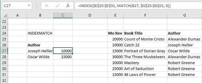
Remember our previous data setup that got our VLOOKUP formula’s feathers all ruffled?? Let’s take another stab at it, this time with INDEX MATCH.

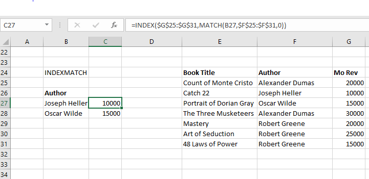
=INDEX(Column to return from, MATCH ( Lookup Value, Column to search, 0)

The index section is used to highlight the range where the values will come from. Inside the match brackets, the user will enter the Value to match and the column to examine. The zero indicates an exact match.

If input correctly this combination formula will return a value from a given range based on a matching value.

Sounds like VLOOKUP, Why should I use INDEX MATCH?

Index Match works very similarly to VLOOKUP but has several advantages. Here are a few:

Ambidextrous – One of the major inconveniences of VLOOKUP is that it only operates if the data you are searching for is to the right of the data you are matching against. It works from left to right and that’s the end of the story! INDEX MATCH can handle multiple looks.

Faster Setup– Once you get familiar with the syntax of Index match, the formula becomes much quicker than VLOOKUP. The main reason is that one row is selected instead of an entire table of data.

Faster Processing– Also related to the user explicitly highlighting a column, Excel can ignore the rest of the table in its computations.

No HLOOKUP Required – Most Excel users are familiar with VLOOKUP which stands for vertical lookup and works its way down columns. If the data is organized horizontally and we need to work across rows the horizontal lookup or HLOOKUP is required. INDEX MATCH is a one-stop solution for all-around lookups.

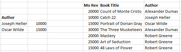
Check out this example of INDEX MATCH Looking left like it’s no big deal!

SUMIF

Earlier when discussing Lookups, we deliberately ignored the situations with duplicate information. There are several ways to sort through duplicated excel information to make them more useable.

However, if the duplicate data is intentional and returning numeric data, the SUMIF function can be very useful.

Let’s look at how SUMIF can be used to lookup values (kind of). The SUM If function adds together certain cells if the criteria are matching. It is well utilized, to sum up, numerical data.

Here’s the syntax of a SUMIF statement:

SUMIF(Cells to apply matching criteria against, Matching Criteria, *Range to Sum up)

*field is optional; if omitted the Cells used to match criteria will be summed.
The range inspected for matches can also be text-based. Just take a look at this example!

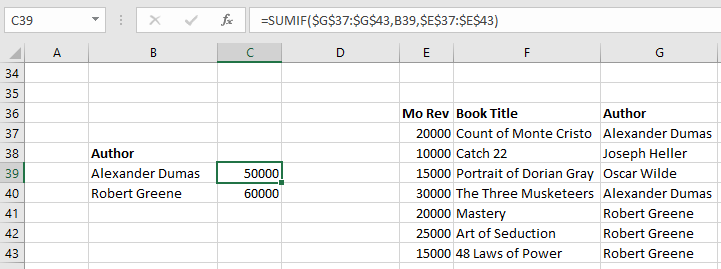
In cell C39 we have the formula: =SUMIF($G$37:$G43, B39,$E$37:$E$43)
This formula looks up the name in the Author field in column B and matches it against the Author in column G. If a Match is found the formula looks to the “Monthly Revenue Column” (Column E) and adds the totals.

Conclusion

Hopefully, someone finds the preceding review of lookups helpful. It’s beneficial to learn multiple approaches to problem solving in excel because the most common methods aren’t always the most efficient. Good luck with your Lookups!